1. Introduction to the CHOOSECOLS Function
When working with data sets containing hundreds or even thousands of columns, it is important to prioritize the most important data. The
CHOOSECOLS function allows you to efficiently retrieve specific information from an array so that you can focus on the most relevant data first.
2. Parameters of the CHOOSECOLS Function
Here is the syntax for using the
CHOOSECOLS function.=CHOOSECOLS(array, col_num1, [col_num2], …)array: required The array containing the columns to be returned in the new array. col_num1: required The first column to be returned. col_num2: optional Additional columns to be returned. 3. Focus on a subset of column data
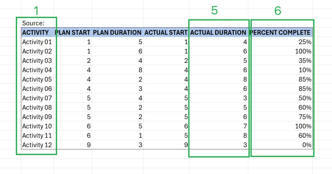
When we have a dataset, it may contain many columns, and we may only want to focus on a subset of those columns. We can use the
For example, here we want to focus on columns 1, 5, and 6.
CHOOSECOLS function to extract this subset of column data in real-time. For example, here we want to focus on columns 1, 5, and 6.
4. Getting Started with the CHOOSECOLS Function
Type on the keyboard:
=CHOOSECOLS(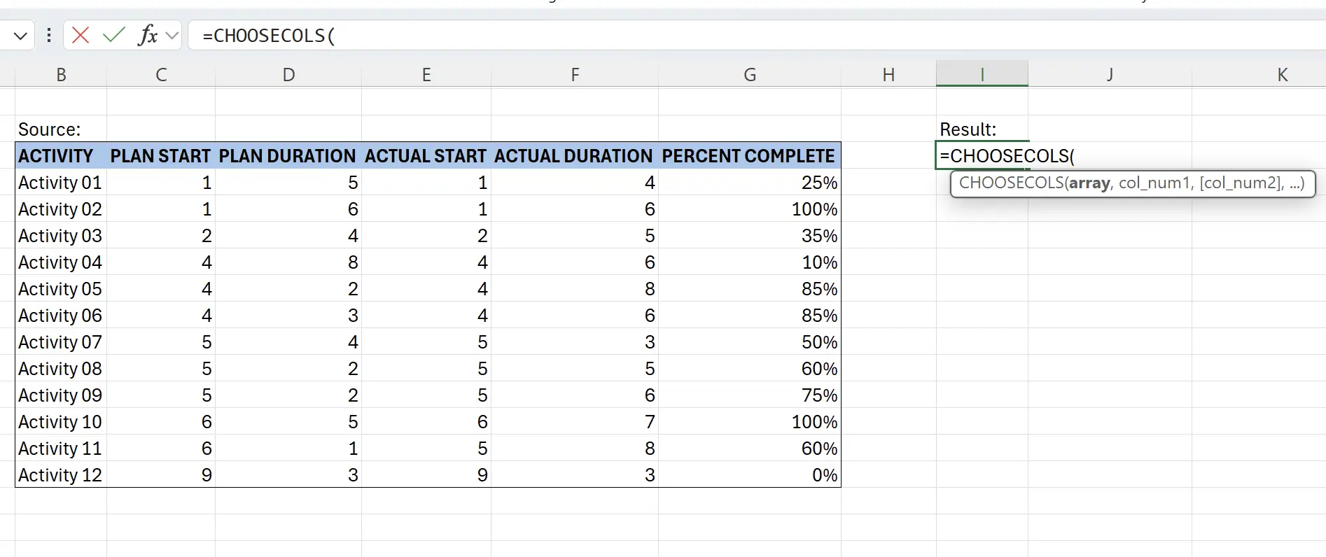
5. Select the source data range
At this point, the function will prompt you to select the source data range. Click on the beginning of the source data
B6, then hold down the Shift key and click on the end of the source data G18. This way, you can select the contents of the source data and fill it into the function parameters: =CHOOSECOLS(B6:G18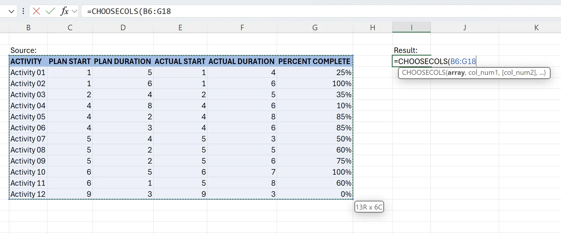
6. Input the columns to extract
Here we enter the numbers: 1, 5, 6, separated by commas, and add the closing
) symbol, resulting in the function: =CHOOSECOLS(B6:G18, 1, 5, 6), then press Enter to save.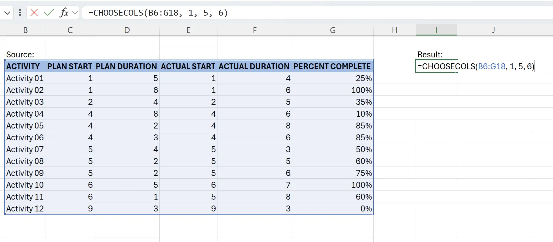
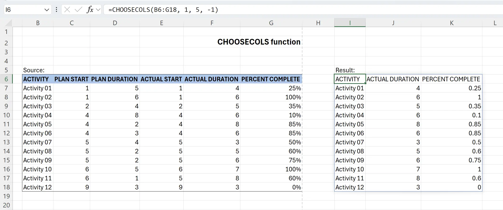
7. CHOOSECOLS function in effect
At this point, we can see the effect of
CHOOSECOLS. It extracts the contents of columns 1, 5, and 6 from the source data in real-time.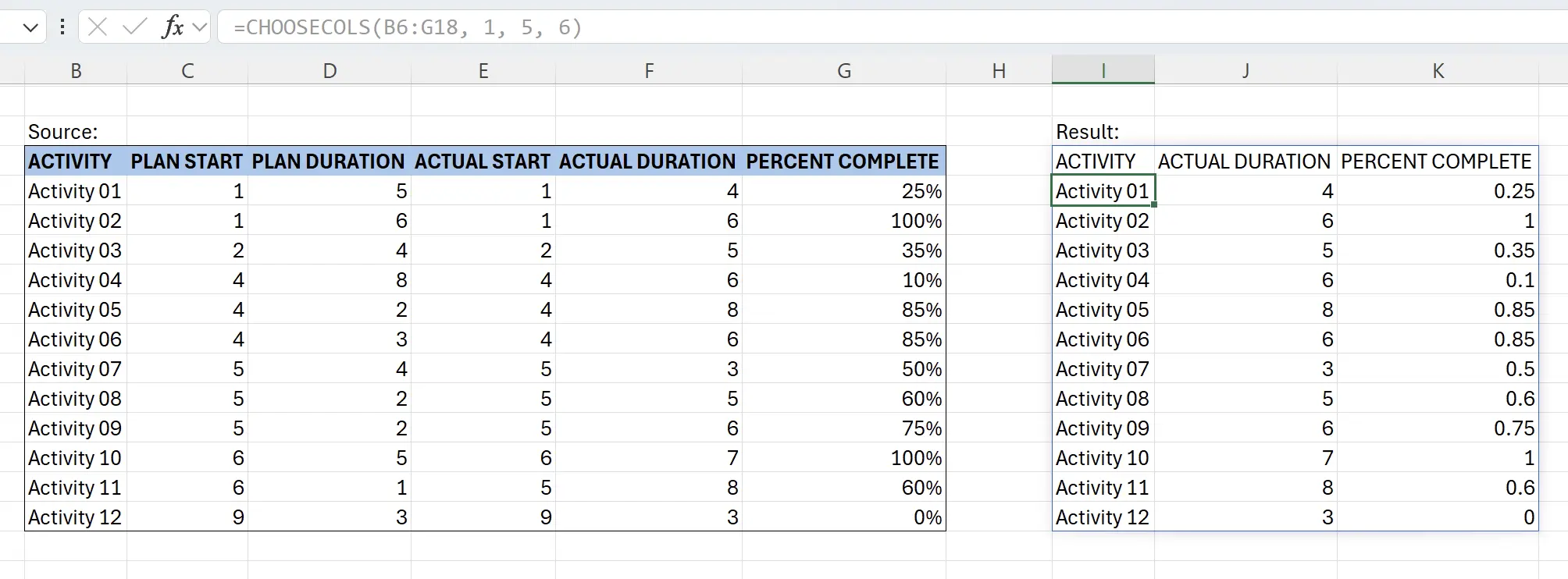
8. Columns can also be represented with negative numbers
The column parameters can also be negative. For example, -1 represents the last column, -2 represents the column before the last one, and so forth. Therefore,
=CHOOSECOLS(B6:G18, 1, 5, -1) will yield the same result.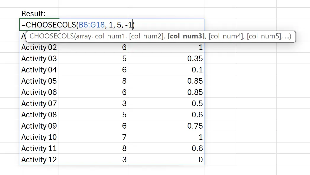
9. 🎉 Finish! 🎉
Author's Note: I hope you can feel the effort I put into these tutorials. I hope to create a series of very easy-to-understand Excel tutorials.If it is useful, help me share these tutorials, thank you!
Follow me:
Related Tutorials
