1. Freeze Panes
Freezing panes in Excel is a key feature that allows users to keep specific rows or columns visible while scrolling through large datasets. This is particularly useful in scenarios where headers contain critical information, providing more context when interpreting data.
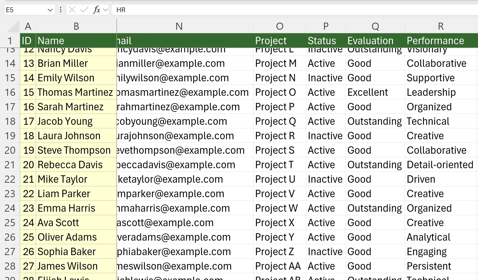
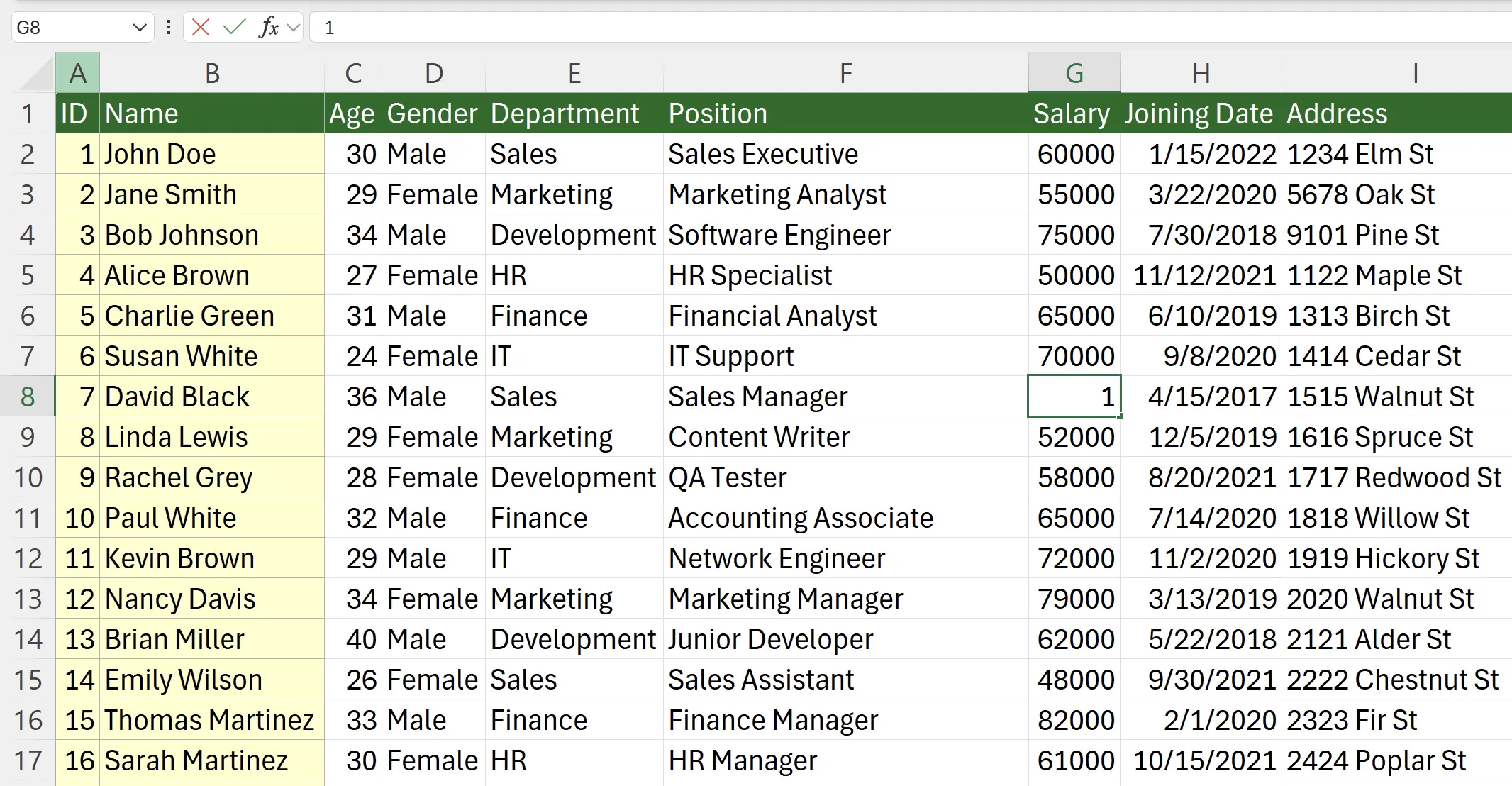
2. Example Scenario
For instance, consider a worksheet with fifty rows and fifty columns. When scrolling through the data, it’s easy to lose track of which column or row a particular cell corresponds to.
3. Apply Freeze Panes
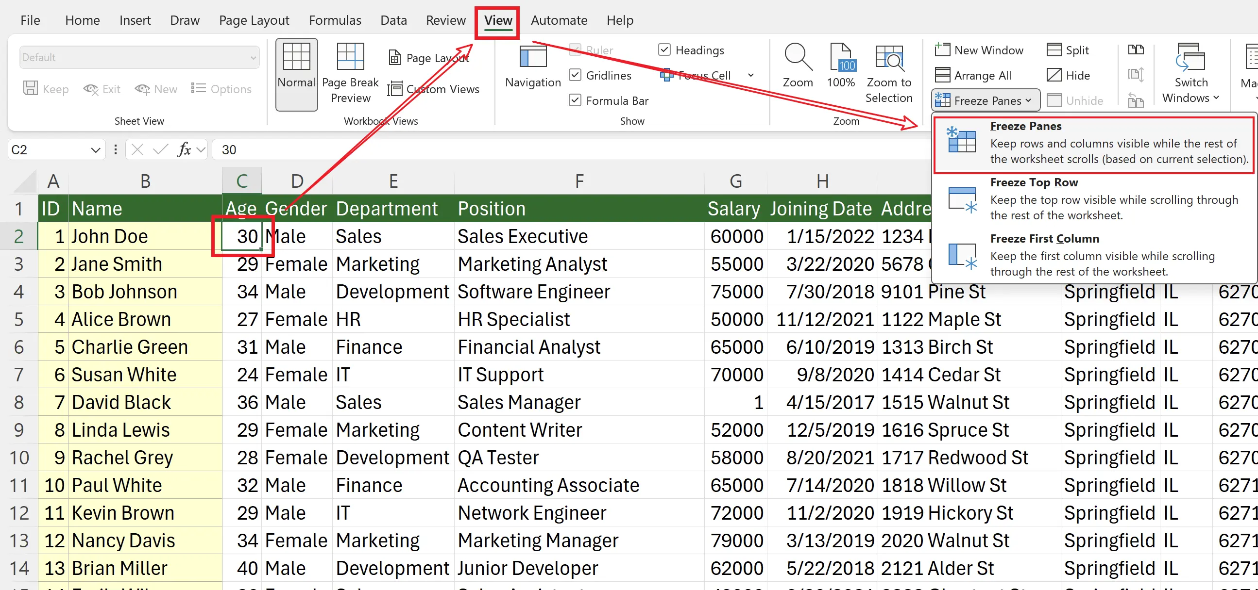
We can select the
Alternatively, we can use the options below to freeze the first row or first column.
C2 cell, then click the Freeze Panes button under the View tab. All columns before C2 and all rows above C2 will be frozen. Alternatively, we can use the options below to freeze the first row or first column.
4. Test the Freeze Effect
Now, try scrolling the worksheet up, down, left, and right. You’ll notice the first row remains fixed at the top, and the first two columns stay fixed on the left.
5. Unfreeze Panes
When we no longer need the panes frozen, we can find the unfreeze option within the
Freeze Panes button under the View tab.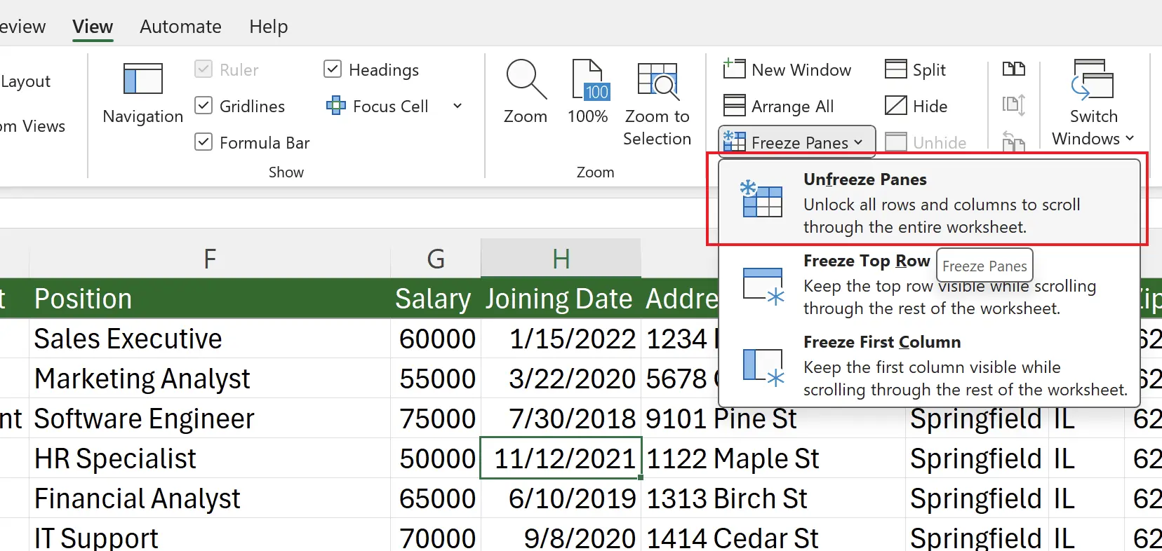
6. 🎉 Finish! 🎉
Author's Note: I hope you can feel the effort I put into these tutorials. I hope to create a series of very easy-to-understand Excel tutorials.If it is useful, help me share these tutorials, thank you!
Follow me:
Related Tutorials